
Statistical Rethinking chapter 2 exercises
Disclaimer
Below are my solutions to the end of chapter exercises in Statistical Rethinking by Richard McElreath.
These results might not be correct, in particular, 2H4 gave me difficulties. If you catch any errors or mistakes please leave a comment below.
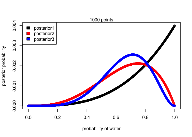
2M1:
First we’ll start off by defining our grid and prior, just make sure the amount of times you repeat the prior is equal to the lenght.out.
Defining the likelihoods uses the dbinom() which stands for density binomial distribution. We start by inputing how many observations were ‘waters’, the size is equal to the total number of tosses, and prob is equal to our grid.
Comupting the posterior is the product of our likelihood and prior divided by the sum of all those values.
# Define the grid
p_grid <- seq(from=0, to=1, length.out = 1000)

# Assume a uniform prior
prior1 <- rep(1, 1000)

# Get the likelihood given: 3 waters and 3 tosses
#                           3 waters and 4 tosses
#                           5 waters and 7 tosses
likelihood1 <- dbinom(3, size=3, prob=p_grid)
likelihood2 <- dbinom(3, size=4, prob=p_grid)
likelihood3 <- dbinom(5, size=7, prob=p_grid)

# Compute posterior
posterior1 <- likelihood1 * prior1
posterior2 <- likelihood2 * prior1
posterior3 <- likelihood3 * prior1

# Standardize
posterior1 <- posterior1 / sum(posterior1)
posterior2 <- posterior2 / sum(posterior2)
posterior3 <- posterior3 / sum(posterior3)

# Plotting the posteriors
plot(p_grid, posterior1, type = "b",
     xlab = "probability of water",
     ylab = "posterior probability")
lines(p_grid, posterior2, type = "b", col = "red")
lines(p_grid, posterior3, type = "b", col = "blue")
legend("topleft",
       c("posterior1", "posterior2", "posterior3"),
       fill = c("black", "red", "blue"))
mtext("1000 points")
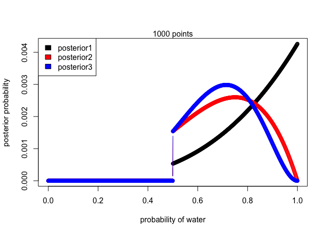
2M2:
This problem is identical to the one above, the only thing that’s changed is that we now our prior, instead of being uniform, is 0 when p < 0.5 and 1 otherwise. This can all be done in r using the ifelse() function.
2M3:
Since earth is 70% water then there’s only a 30% or 0.3 chance that it will land on ‘land’. Mars has a 100% or 1.0 chance of landing on ‘land’ if tossed.
Below are two identical ways of solving the problem, the second was included in case it’s not as clear how the code in the first part works.
ways <- c(.3, 1)
probability <- ways/sum(ways)
probability[1]
## [1] 0.2307692
# Alternative way
earth_land = 1-.7
mars_land = 1
probability_earth = earth_land/(earth_land + mars_land)
probability_earth
## [1] 0.2307692
2M4:
For the following set of questions I’ll be using [bb], [bw], and [ww] to refer to a card that is black on boths sides, black on one side/ white on the other, and white on both sides.
If [bb] is picked there’s a 100% or 1.0 chance that when it’s put on the table a black side is facing up. If [bw] is picked it’s a 50% or 0.5 chance. If [ww] is picked there’s a 0% chance that a black side can be facing up.
Another way of thinking about it is there are two ways a [bb] card can show a black side up, only one way a [bw] card can, and no ways for a [ww] card.
ways <- c(1, 0.5, 0)
probability <- ways/sum(ways)
probability[1]
## [1] 0.6666667
# ways <- c(2, 1, 0)
# p <- ways/sum(ways)
# p[1]
2M5:
Now there is an extra [bb] card. I like thinking about this in terms of percentages, so there are two cards that have a 100% chance of showing a black side face up, everything else is the same from 2M4.
Alternatively, as in 2M4, you can think of it as there are two ways a [bb] card can show a black side face up, one way for a [bw] card, no ways for [ww], and again two ways for the second [bb] card. Since we can pick either of the [bb] cards we add their probabilities together to get the final result.
ways <- c(2*1, 0.5, 0)
probability <- ways/sum(ways)
probability[1]
## [1] 0.8
# ways <- c(2, 1, 0, 2)
# probability <- ways/sum(ways)
# sum(probability[1], probability[4])
2M6:
Now we are informed that for every way we can pull [bb] there are two ways we can pull [bw] and three ways to pull [ww]. In the previous examples we were making the implicit assumption that there were equal chances of drawing each card meaning that our prior was uniform, i.e. 1 for each card. Now we need to adjust our probability given this new prior.
# You could also use: ways <- c(2, 1, 0)
ways <- c(1, 0.5, 0)
prior <- c(1, 2, 3)
likelihood <- ways * prior
probability <- likelihood/sum(likelihood)
probability[1]
## [1] 0.5
2M7:
To solve this problem we’ll look at all the possible combinations of draws that can lead to a black side showing face up on the first draw followed by a white side showing up on the second. Since a [bb] card has two ways it can show a black side face up, I will introduce a new notation [Bb] and [bB] to represent the two different states of the same card. The same logic will be applied to [ww], [bw] need not change because there’s only one way a [bw] card can show either black or white.
| First Draw | Second Draw |
|---|---|
| Bb | bw |
| Bb | Ww |
| Bb | wW |
| bB | bw |
| bB | Ww |
| bB | wW |
| bw | Ww |
| bw | wW |
From this we can see that there are six ways a [bb] card can be picked first, and only two ways for the [bw] card to be picked first. There are still no ways a [ww] could be picked first.
ways <- c(6, 2, 0)
probability <- ways/sum(ways)
probability[1]
## [1] 0.75
2H1:
The relevant information here is that the probability of a panda giving birth to twins given that it’s from species A is 10% and species B is 20%. Also, that both species of panda are equally common so. From this we know the following:
Using Bayes Theorem we can find the following:
likelihood <- c(0.1, 0.2)
prior <- c(1,1)
posterior <- likelihood * prior
posterior <- posterior/sum(posterior)
posterior[1]
## [1] 0.3333333
From this we know that
Now we can calculate Pr(twins)
0.1*posterior[1]+0.2*posterior[2]
## [1] 0.1666667
2H2:
We actually already computed this in our solution above:
posterior[1]
## [1] 0.3333333
2H3:
Since we know the probability of each species giving birth to twins, we can assume that the probability of giving birth to a singleton is just the complement of our previous probabilities. Therefore:
Since we’re assuming that the first birth were twins, we can reuse our probabilities for A and B.
Now we can use Bayes Theorem again to solve the problem:
likelihood <- c(0.9, 0.8)
prior <- c(1/3, 2/3)
posterior <- likelihood * prior
posterior <- posterior/sum(posterior)
posterior[1]
## [1] 0.36
2H4:
I want to preface that this question gave me some trouble, I’ll do my best to explain my thought process but if anyone has any feedback please let me know.
We know that the probability this test correctly identifies a panda from species A is 0.8, we also know that the probability that this test correctly identifies a panda from species B is 0.65. I’ve included the following type error chart to help visualize the test.
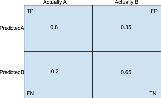
We can interpret this as
Since TP + FN = 1 and FP + TN = 1 we can see that
I hope the chart above helps illustrate why this is the case. Now back to the question. For the first part we will be ignoring the information from the previous questions and focus on computing the posterior probability that the panda is from species A given that the test results say it’s species A.
likelihood <- c(0.8, 0.35)
prior <- c(1, 1)
posterior <- likelihood * prior
posterior <- posterior/sum(posterior)
posterior[1]
## [1] 0.6956522
Now we will use the birth data
likelihood <- c(0.1, 0.2)
prior <- c(0.696, 0.304)
posterior <- likelihood * prior
posterior <- posterior/sum(posterior)
posterior[1]
## [1] 0.5337423
Comments